In the first half of the guide, we examined a series of tools that are useful for increasing the precision and quality of rendering in order to push ourselves to the threshold of photorealism. As we delve into the mechanisms of animation, we may therefore desire a similar realism for what concerns the movement of objects. For example, if we wanted to animate a bowling ball hitting bowling pins, it would not be convenient to search for all the necessary set of keyframes and interpolations to approximately make the sequence realistic. Blender provides the tools to simulate physical dynamics for various types of bodies and systems, to the level of precision that we desire. The bowling case falls under the dynamics of rigid bodies, so called because they maintain their geometric structure unchanged regardless of motion and impacts. If, on the other hand, we had to represent a deflated ball that deforms by hitting other bodies? In that case, we would resort to Soft Bodies. If we were interested in simulating the behavior of a flag, a sheet of paper, or a garment? We have the possibility to adopt the Cloth tool.
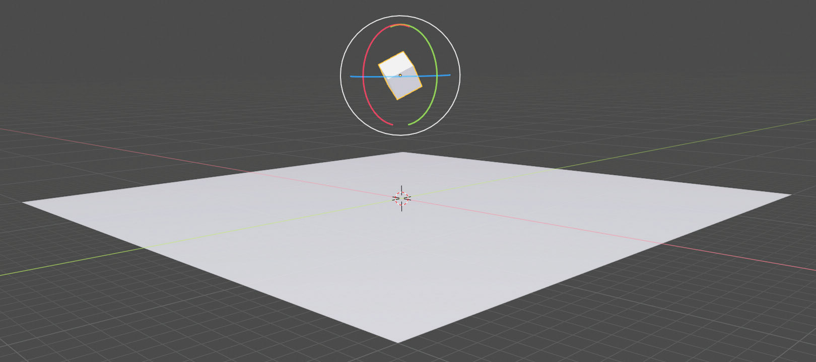
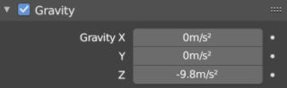
Let’s start getting familiar with the physics of rigid bodies by observing the cube (rotated as in the image above) falling onto a plane due to gravity. The gravitational acceleration along the Z (global) axis is the only one that will act on the cube in this example; its intensity is defined in the Scene properties context, under the ![]() icon
icon
Select the plane and go to the Physics properties context, under the ![]() icon.
icon.
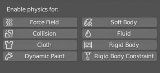
For the plane, just activate (by clicking on the respective button) the Rigid Body dynamics.
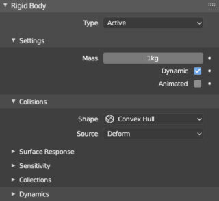
Since the plane will have to remain stationary as a “floor” and not fall into the void due to the force of gravity, we change the first entry at the top from Active to Passive, with this choice many of the previous options will disappear. We perform the same exact operations on our cube, leaving the rigid body dynamics active and all the default settings. At this point, by clicking Play in the timeline (space bar), we will see the cube fall due to gravitational attraction. Having rotated the mesh in such a way as to make it impact on one of its own edges, the animation calculated in real time by Blender will be such as to convince us that only with great difficulty and patience we would have been able to obtain a similar result through the use of keyframes. Let’s see then what happened to the timeline after Blender calculated our animation.
![]()
As you can see, an orange line has appeared under the entire range of frames. This means that Blender has calculated and stored in a cache the movements of all bodies with physical dynamics. If the scene were very complex, and the calculations of the physics engine were quite heavy, you would only have to wait once for the time needed to store all the data, and then see the precalculated animation unfold at the frame rate we set (unless the graphic representation in the preview is also heavy enough to cause some slowness). Obviously, by changing the initial conditions, such as moving the cube, Blender will recalculate the entire dynamics of the scene when the animation is restarted. The data cache for the rigid body is located in the Scene context where we find the Rigid Body World panel: a set of options related to the RigidBodyWorld collection, which automatically includes all bodies to which we have assigned this dynamics.
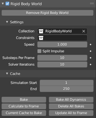
We will see in detail the simple functioning of the Cache by studying Soft Bodies and Cloths, for which the amount of calculations is definitely higher than animations that only involve rigid bodies. It is not certain that the physical animation in Blender will immediately return the desired result, it may in fact happen to observe a completely wrong, imprecise and error-filled behavior. This is because, depending on the type of scene to be animated, it will be necessary to properly adjust the various parameters and possibly also refine the calculation precision. The main way is therefore, in this case as well, trial and error and the accumulation of experience in experimenting with different situations. To increase the calculation precision, go to the Setting panel where we find the values Substeps Per Frame (0-1000) and Solver Iterations (10-100) to be increased for greater precision. The Speed parameter (located in the same panel) is very interesting, as it is used to accelerate or slow down the simulation, even dynamically, using keyframes. We can, for example, slow down the action (up to stopping it) at a “topical” moment, simulating the suggestive effect of “Bullet Time” (perhaps increasing the calculation precision precisely at that specific moment).
Let’s now delve into the important physical phenomena of elasticity and friction of rigid bodies. As you have seen from the first example of physical dynamics of the cube, it did not bounce off the plane but simply settled on one of its faces. In the options of the rigid body dynamics (Physics properties context) Rigid Body panel > Surface Response, we find the two parameters Friction (default at 0.5) and Bounciness (default at 0), the latter is linked to elasticity.
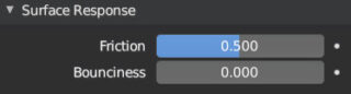
However, even by setting this parameter to the maximum, the result of the animation will not change. In fact, to obtain a change, it is necessary to increase the Bounciness also for the plane, that is, for both the two colliding surfaces. By setting these values to 1, you will notice that the cube will tend to bounce and not completely stabilize until after several frames (especially if it tends to bounce on its own edges). If in addition to this we set friction to 0 for both bodies, the motion of the cube may not stop within the range of frames. Why does this happen? The reason is that Friction and Bounciness regulate the behavior of collisions between objects, including the dissipation of the kinetic energy of a moving body. In reality, during collisions between bodies, there is always a transformation of the original kinetic energy into other forms of non-mechanical energy such as heat; in practice, this is the phenomenon that prevents the existence of perpetual motion. One of the causes that determines the dissipation of the kinetic energy of bodies is the friction between two surfaces; let’s immediately verify what has just been said with a practical example (you can use Blender as a small virtual physics laboratory). We start from the primitive UV Sphere with rigid body dynamics, ready to fall onto an inclined plane.
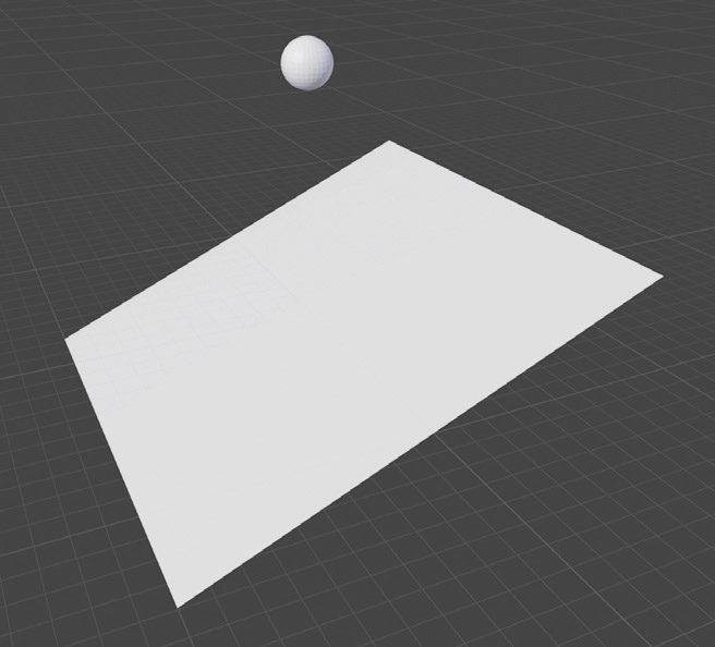
We assign a passive rigid body dynamics to the plane again, while for the sphere it is active. Also in this case, the default values for Friction and Bounciness return the realistic behavior of a rigid spherical body, which after impacting will roll on the plane and then fall into the void. Now we change some settings of the sphere by zeroing out friction and choosing Sphere in the Shape field of the Rigid Body panel > Collisions.
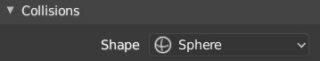
In this way, our sphere, after hitting the plane, will slide on it instead of rolling. In fact, the rotational-translational movement of a sphere along an inclined plane occurs precisely due to the phenomenon of friction, in turn generated by the interaction between two different surfaces. So why did we insert Sphere in Rigid Body > Collisions, in the Shape field? The Blender physics engine has several ways of considering the shape of the object during a collision:
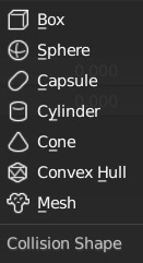
- Mesh, the Blender physics engine calculates collisions based on the exact polygonal structure of the object.
- Convex Hull is an approximation of the original shape obtained with a few polygons.
- Cone, Cylinder, Sphere and Box, exactly what the names say.
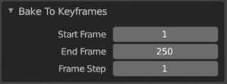
By choosing sphere, it will not matter the level of detail of the UV Sphere, as the Blender physics engine considers the object as a perfectly curved sphere. In fact, for any other choice, the sphere would not have slipped along the plane, despite the null friction parameter, because it is not geometrically “smooth”, but made up of a discrete set of single faces that would have determined its rolling. Applying a Collision Shape of type Sphere to any rigid body, such as the primitive monkey mesh (suzanne), will also roll as if it were inside an invisible sphere (depending on the friction parameters). The options in Collision > Shape are therefore different approximations that will be chosen according to the circumstances. Once your animation is complete, you can transform the entire action into keyframes through the Bake to Keyframes located in the Object menu > Rigid Body of the 3D View.
If any of you decide to take up the invitation to start experimenting with Blender’s physics simulation, you will soon realize a lack; that is, in the various options for rigid bodies it is not possible to set any value for the initial velocity of the objects, let alone the angular velocity. Of course, we cannot always start simulations with stationary bodies because in the absence of gravity or any other force field, nothing will happen. So let’s see how to do it: in the Rigid Body>Settings panel of the physics context we notice that under the Dynamic box (active by default) is the other box Animated, initially inactive.
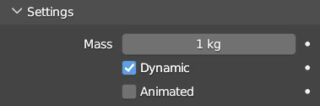
With the activation of Animated, the physical dynamics will be excluded (except for collisions) and the object will be forced to behave as indicated through keyframes. If no keyframes are set, the object will remain still throughout the simulation. So at the first frame we can set both a Location & Rotation keyframe for the rigid body and an active Animated box keyframe ![]() then, in a second frame (even a few frames later), we will translate the cube in the direction of the initial velocity we want and rotate it by a chosen angle (around any axis), here we will insert another Location & Rotation keyframe for the rigid body and finally the last keyframe for the deactivated Animated box
then, in a second frame (even a few frames later), we will translate the cube in the direction of the initial velocity we want and rotate it by a chosen angle (around any axis), here we will insert another Location & Rotation keyframe for the rigid body and finally the last keyframe for the deactivated Animated box ![]() .
.
When starting the animation you will see the cube initially move between the two LocRot keyframes as per interpolation, while from the next frame the physical simulation will begin in which our cube will have an initial velocity (spatial and angular) based on the motion that took place between the two keyframes. The greater the distance traveled by the rigid body between one keyframe and the other, the greater the initial velocity for the physical simulation (the same is true for angular velocity).
To conclude the topic on the motion of rigid bodies, let’s see the Rigid Body>Dynamics panel.
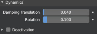
In particular, the two values Damping Translation and Rotation. By increasing these values, we will reduce (damping = dampen) the ability of bodies to translate and rotate independently of external stresses.
Next paragraph
Previous paragraph
Back to Index
Wishing you an enjoyable and productive study with Blender, I would like to remind you that you can support this project in two ways: by making a small donation through PayPal or by purchasing the professionally formatted and optimized for tablet viewing PDF version on Lulu.com