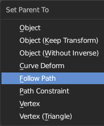
When animating an object through keyframes of location and rotation, perhaps diversifying the interpolation for the individual spatial coordinates and/or rotation angles, we will create a path within the 3D space along which the object will also rotate around its own origin. If we already have a particular trajectory in mind, we can define this path by modeling a curve and then “constraining” the object to follow it along its orientation. The curves that we will adopt as paths are ![]() that is, flat and straight NURBS curves by default. The object that will be animated along a predefined path in this paragraph will be our camera, as the typical use of this animation technique concerns the movements of the camera within a scene. We define the path by modifying the path curve through its control points, modeling it, for example, in the top ortho view (in which case it will remain flat). We place the camera in a way that it is already prepared to follow the path according to its orientation (visible in Edit Mode as mentioned in paragraph 2.4) and after selecting the camera first and then the NURBS, we launch the parenting options menu with Ctrl-P, choosing Follow Path.
that is, flat and straight NURBS curves by default. The object that will be animated along a predefined path in this paragraph will be our camera, as the typical use of this animation technique concerns the movements of the camera within a scene. We define the path by modifying the path curve through its control points, modeling it, for example, in the top ortho view (in which case it will remain flat). We place the camera in a way that it is already prepared to follow the path according to its orientation (visible in Edit Mode as mentioned in paragraph 2.4) and after selecting the camera first and then the NURBS, we launch the parenting options menu with Ctrl-P, choosing Follow Path.
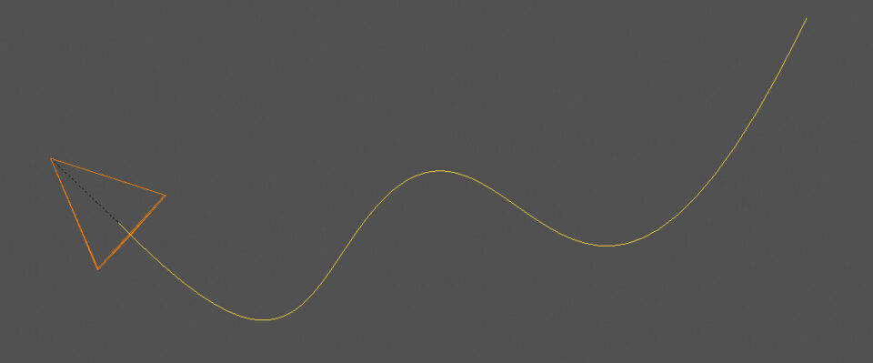
We will see the dotted line appear that highlights the child (camera) > parent relationship.
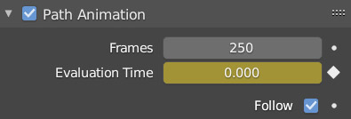
Before launching the animation, we select the curve and go to the Object Data context by clicking on the properties icon ![]() here in the Path Animation panel
here in the Path Animation panel
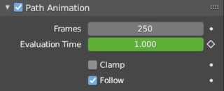
We need to replace the default value of Frames from the default 100 to the number of frames that interest us, then you can start the animation. Observing the Path in edit mode we notice that the arrows are parallel to the plane to which the curve belongs unless a control point is translated along the z-axis.

We select a control point and go to act on the Tilt parameter located in the sidebar of the 3D View (key N), Item tab, Control Point panel.
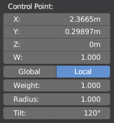
Through Tilt we can rotate the orientation of the arrows and see a screwing of the path simply by typing the rotation value in degrees. Restarting the animation from the camera’s point of view, we will see that at the control point the view will rotate by an inclination corresponding to the value we decided in Tilt. For this type of animation we have not yet set any keyframes, and if we want a motion with varying speeds, even to the suspension of movement, we must use the Graph Editor, but only after one more step. First, let’s see how the Graph Editor looks by selecting the path curve (and not the camera).
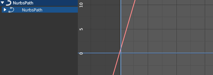
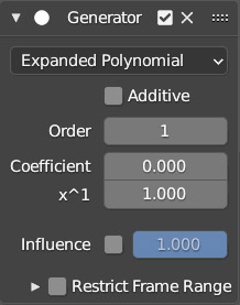
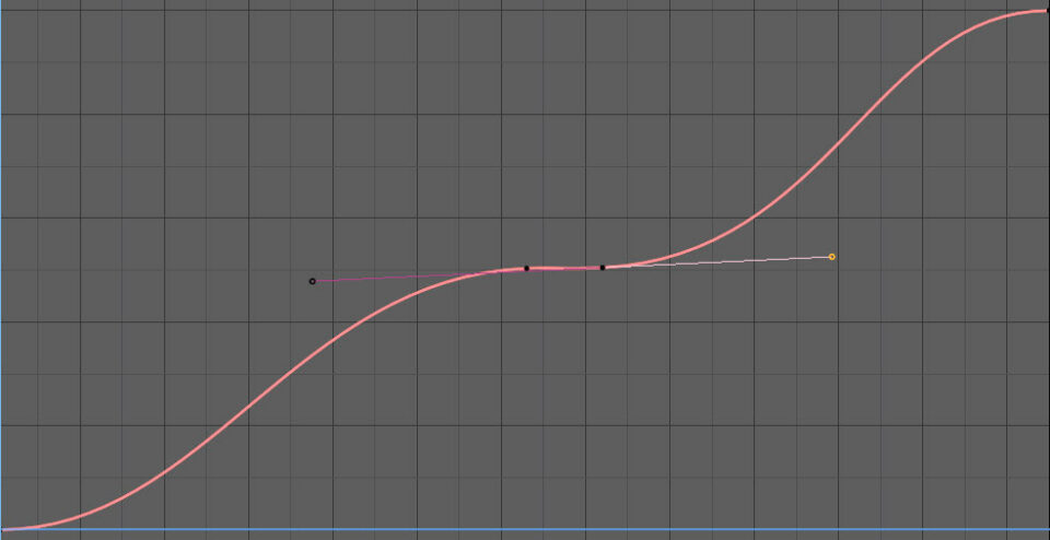
We find a straight line (constant speed motion), top image, which is not actually the classic interpolation between two keyframes that we know, as we have not yet fixed any keyframes as mentioned before. By checking in the Graph Editor sidebar, Modifier tab, we will discover that this line is generated by the Generator/Expandend Polynomial modifier, with which it is possible to create functions of the type: y(x)=ax+bx2+cx3 (by default y=x).
But don’t worry, we can delete this modifier by clicking the x in the top right and see how to go back to manipulating an interpolation curve as seen in the previous paragraphs. We return to the Path Animation panel and in the first frame of the animation we fix a keyframe for Evaluation Time equal to Zero.
Then we go to the last frame and fix a keyframe for Evaluation Time equal to the number of our frames. Restart the animation and we will see that it will be completed along the path with the classic Bézier interpolation, which will now be in plain sight in the Graph Editor.
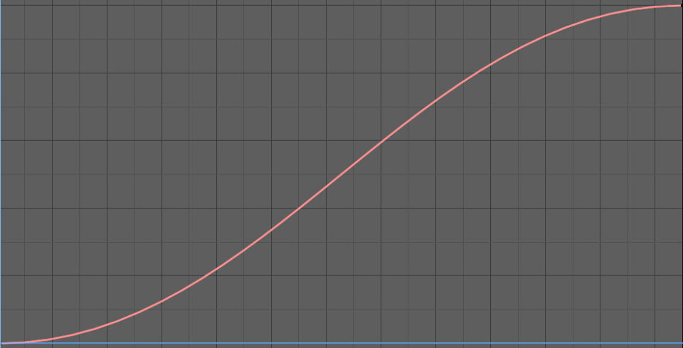
At this point we will be able to define the motion as we see fit, for example by creating a pause point in which the camera will stop for a moment.
A need that is usually had when animating the camera along a path is to make it consistently point at another object or area in space, as in the images on the top right. So we enter the context of Constraints of the properties, icon ![]() where clicking
where clicking ![]() will open a rich menu containing all the constraints.
will open a rich menu containing all the constraints.
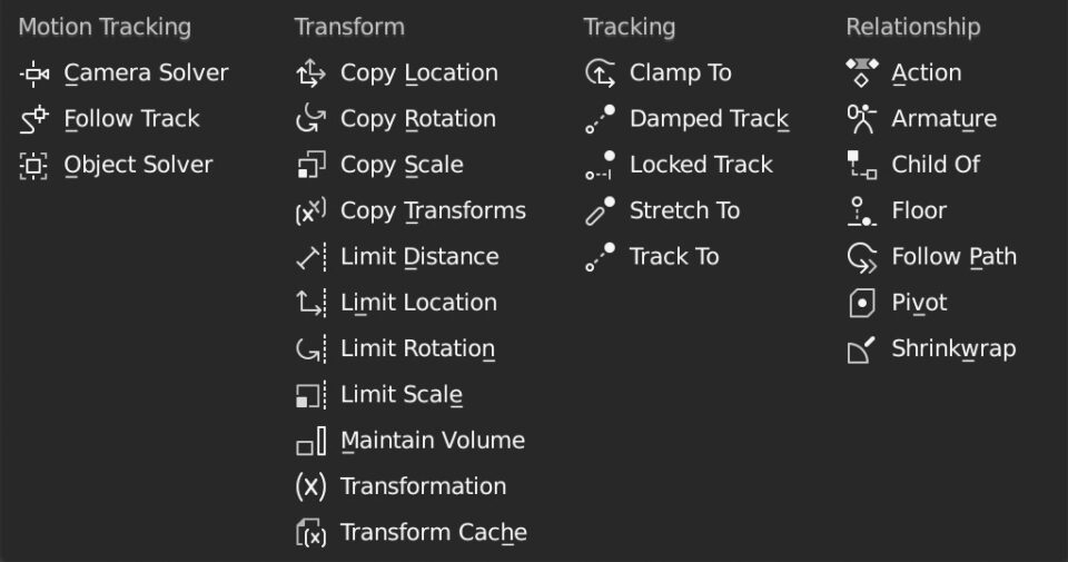
Constraints enrich our ability to establish binding relationships between objects, particularly useful in animations. We select Track To (Tracking category) and set it up exactly as in the image.
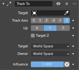
so in Target, we will insert the object that the camera will have to fix. In To we select -Z, then Y in Up. The X Y and Z axes indicated in To and Up are to be understood as belonging to the local reference of the Camera, where the Z (local) axis is in fact the direction in which the camera observes. Y in Up, as the name suggests, is the “up” direction from the camera’s perspective. The Influence parameter, which is set to one by default, can be lowered to gradually release the camera from pointing at the object. By varying the value in influence, through keyframes, we can make the camera point to an object at a specific frame (influence=1) and then return to follow the path (influence=0), or point to another object using another Track To type Constraint.
Let’s delve deeper into some of the transform family constraints (bindings) in particular.
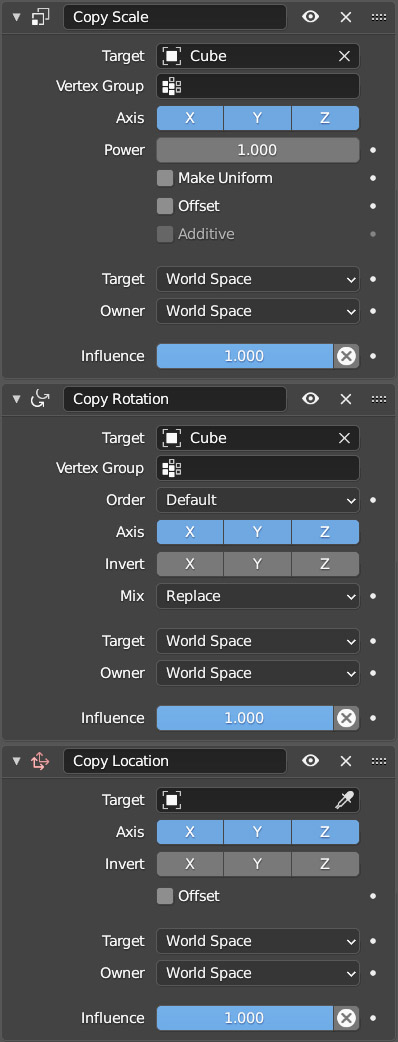
The first four constraints in the Copy series are easy to understand and are generally useful in various types of animation (with or without physical simulation). With these constraints, we can dynamically apply the transformations of one scene element to any object without establishing any parent-child relationship between them. In the Copy Location/Rotation/Scale constraints, we first need to select the element from which to inherit the transformations, which by default are understood in the global orientation (world space <> world space); then we can choose transformations that only affect one or two of the three x, y, z axes, and possibly invert them. By default, the Offset box is not checked, which means that our object will immediately receive the position, rotation, and scale of the target. However, if the offset is activated, the transformations suffered by the target will be applied to the original state of our object. A few experiments will quickly show the functioning and usefulness of these three constraints.
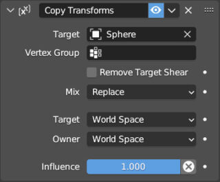
Copy Transforms will not distinguish between types of transformation and will replicate the same transformations applied to another object on any object.
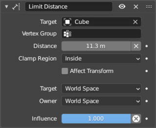
Let’s move on to the four constraints in the Limit series, which are also fairly intuitive. Limit distance (Clamp Region > Inside) forces an object to stay within a spherical surface centered on the element indicated in the target field and with a diameter equal to the value of distance, or, if Clamp Region > Outside is set, the object will be forced to stay outside of this spherical surface, while with Clamp Region > On Surface, the object can only move on the surface. For the distance between two meshes, it is obviously the distance that separates the two origins, and it is the origin of the object with the limit constraint that will be constrained within, outside, or on the surface of the sphere with a radius equal to distance.
The three Limit Location/Rotation/Scale constraints are used to define a range of validity for the respective transformations, beyond which the object cannot be translated, rotated, or scaled.
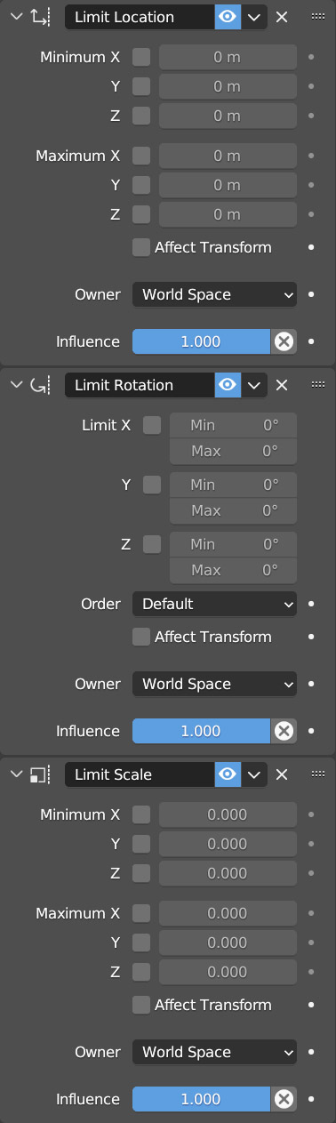
The transformations should be understood in the Global (World space) or Local reference. You just need to set minimum and maximum values for the x, y, and z axes. By setting the Limit Location constraint to: 10 (minimum) and +10 (maximum) for x, y, and z (world space), the origin of the object will be constrained to stay within the cubic volume of side 20 centered at the origin. Be careful because these constraints are maintained only visually, when in reality the actual position, rotation, and scale values are free to vary without any limitation; this is why subsequently deactivating the constraint (eye icon) or deleting it, the object may be in a completely different condition. In the limit rotation constraint, the Min and Max values are indicated in degrees. If the initial rotation for the z axis (world space) was 0, for example, setting a minimum value of 10 and a maximum value of 20, the object will be automatically rotated by 10°.
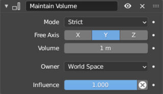
Maintain Volume preserves the volume of a mesh in the Scale transformations performed along the free axis, in either world space or local reference. Using three constraints, one per axis, the volume of the object remains unchanged regardless of the transformation.
Next paragraph
Previous paragraph
Back to Index
Wishing you an enjoyable and productive study with Blender, I would like to remind you that you can support this project in two ways: by making a small donation through PayPal or by purchasing the professionally formatted and optimized for tablet viewing PDF version on Lulu.com