In this paragraph we will see how to complete the definition of materials through the fundamental process of Texturing, that is the technique that increases the detail of the models through the use of textures or textures to be “mapped” appropriately on the surface of the mesh. We start from the base color of the Principled Shader for which so far we have set a uniform RGB color for the entire surface. By applying a bitmap texture (jpg or png) as you can see on the right, the rendering engine will use the rgb / rgba values of the individual pixels of the image loaded in the Image Texture node to map the surface of the model (which in this process is divided into texture elements) this by using an interpolation useful for improving visualization when the surface is close to the camera.

While working with the Principled Shader, we saw that in the definition of a material, most of the parameters are numerical (gray sockets), which is why we can use textures that will not work as RGB color maps, but as intensity maps and used by the rendering engine to vary the numerical parameters point by point on the surface of the model. With these Intensity Maps, graphically represented in a gray scale (256 levels), we will quickly obtain surprising results, such as altering the shading of the surfaces to simulate the presence of reliefs (bump) without having to modify or add even one vertex to our mesh, thus simplifying our modeling phase. The main families of Textures that we will use in Blender are the procedural textures and the bitmap images. Procedural textures are images generated by fractal algorithms that return more or less complex shapes, variable by acting on some parameters. The main advantage of such textures is certainly their very high detail without any need to store data on the hard drive, as they are generated and managed internally by Blender. Compared to Bitmap images, procedural textures will adapt more easily and naturally to the shape of the mesh and are native seamless (i.e. without cuts or discontinuities). An important function of procedural textures is to help us simulate some existing textures in nature, such as clouds, the veins of marble and wood, etc. Each of these will be represented by a node that we can insert in the Shader Editor directly from the Add> Texture menu.
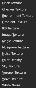
Of those listed, we are interested in all except: IES, Point Density, and White Noise. We apply the Voronoi texture as in the figure below. It is a cell-structured texture that is a bit difficult for the beginner to approach, similar to a random mosaic, but is used in the creation of many materials, from organic fabrics to rough metals.
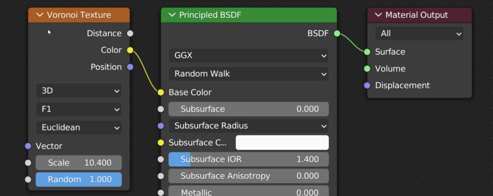
The Distance socket returns a grayscale scale to be used as an intensity map. In the node you can choose the type of grid structure starting from Euclidean (the 3D setting is typical for many procedural textures). You will notice that the graphics engine tends to take a few seconds to display the texture, as it is generated by the CPU, converted to a bitmap, and finally mapped in the real-time view. This is an extremely important feature of Eevee, as without it we would have had to do everything manually through a texture baking process.
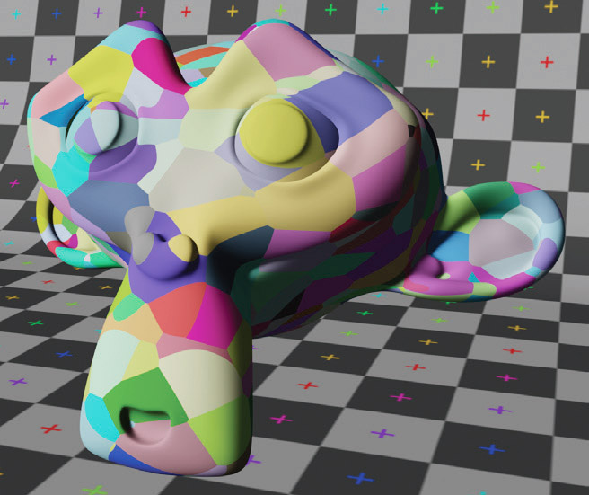
By default, Blender maps textures using Generated coordinates, which we will mainly use when working with procedural textures unless we are looking for particular effects. Let’s now insert the Texture Coordinate and Mapping nodes as shown in the following image.
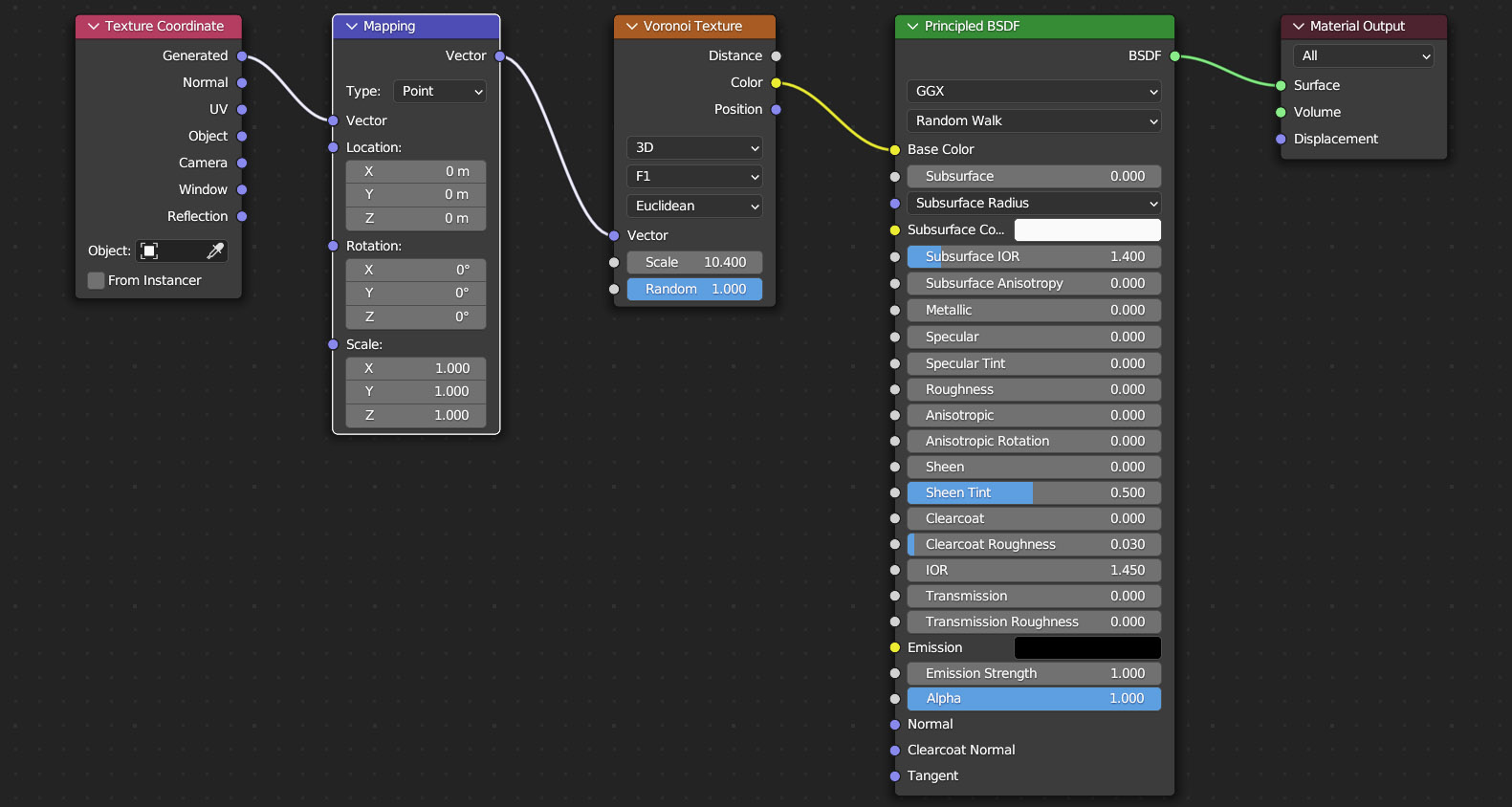
With the coordinates: Window, Reflection, and Camera, the mapping will depend on the position of the mesh in space or the viewing angle. It will only take a few minutes of experimentation to understand the effects of these three systems. Generated has the advantage of processing the texture while staying aligned with the object itself and satisfactorily mapping procedural textures regardless of the geometry of the mesh. With Object coordinates, we can specify another object as the source of the coordinates. We will delve deeper into UV coordinates when discussing Bitmap Textures, a context in which some projection modes (located in the image node) are also useful. After choosing a coordinate system, we can use the mapping node to translate, rotate, and scale the texture along the x, y, and z axes. Let’s now try using the Musgrave procedural texture instead of Voronoi in the same node schema visible above.
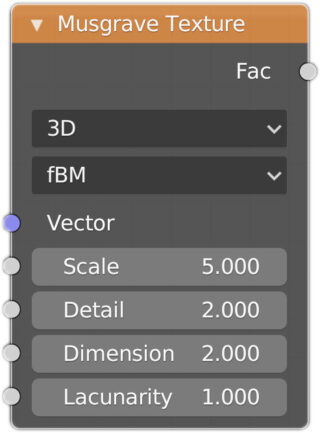
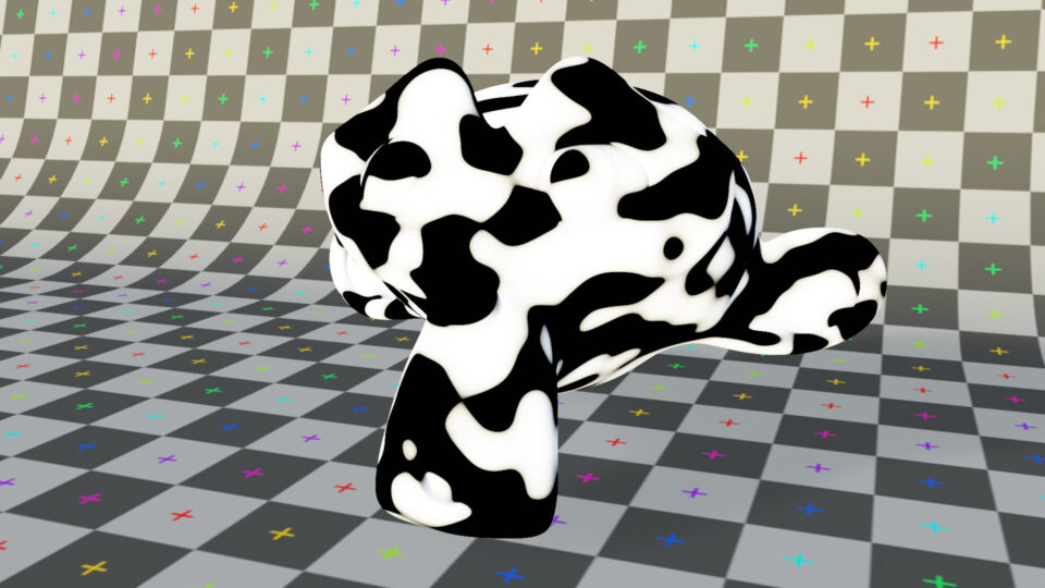
Musgrave is a texture useful in simulating organic matter with five possible fractal formulas (by default you will find fBM fractal Brownian Motion). The node does not have a color output socket (yellow), it is in fact an Intensity Map that must be used differently and for a multitude of different purposes. First, try connecting the Fac output socket (gray) to the input socket (yellow) of the Base Color, and you will see white-black spots on the model.
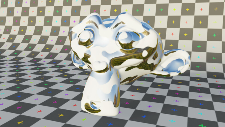
After this, associate the numeric value 1 with the color white and the value zero with the color black in your mind. All intermediate shades will therefore have a value between 0 and 1. At this point, we use the texture by connecting the gray Fac socket to the same color sockets of the Principled Shader. Here is the effect obtained using the intensity map to vary the Metallic value:
or the Transmission value:
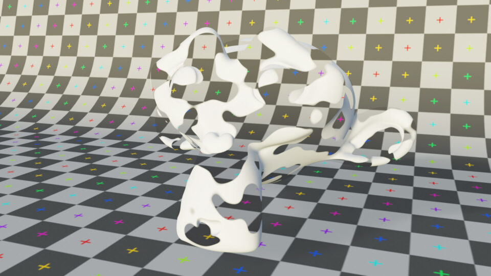
In the latter case, I set the IOR to 1 in order to have pure transparency (remember to activate screen space reflection + refraction in the render context and in the material context). In this way, it is possible to make a mesh partially reflective or transparent (in the areas previously mapped with white) without having to intervene on the structure of the model itself. Imagine how difficult it would have been to remove the transparent parts of the mesh so precisely, or to attribute only to them a reflective material.
With intensity maps, we can increase the complexity of the model to our liking, both by keeping the number of vertices unchanged (bump / normal map) and by drastically increasing the definition of the mesh (displacement). Let’s analyze the material visible in the image below: we find the Noise texture connected to the Bump node (roughness / protrusion) which belongs to the Vector node family.
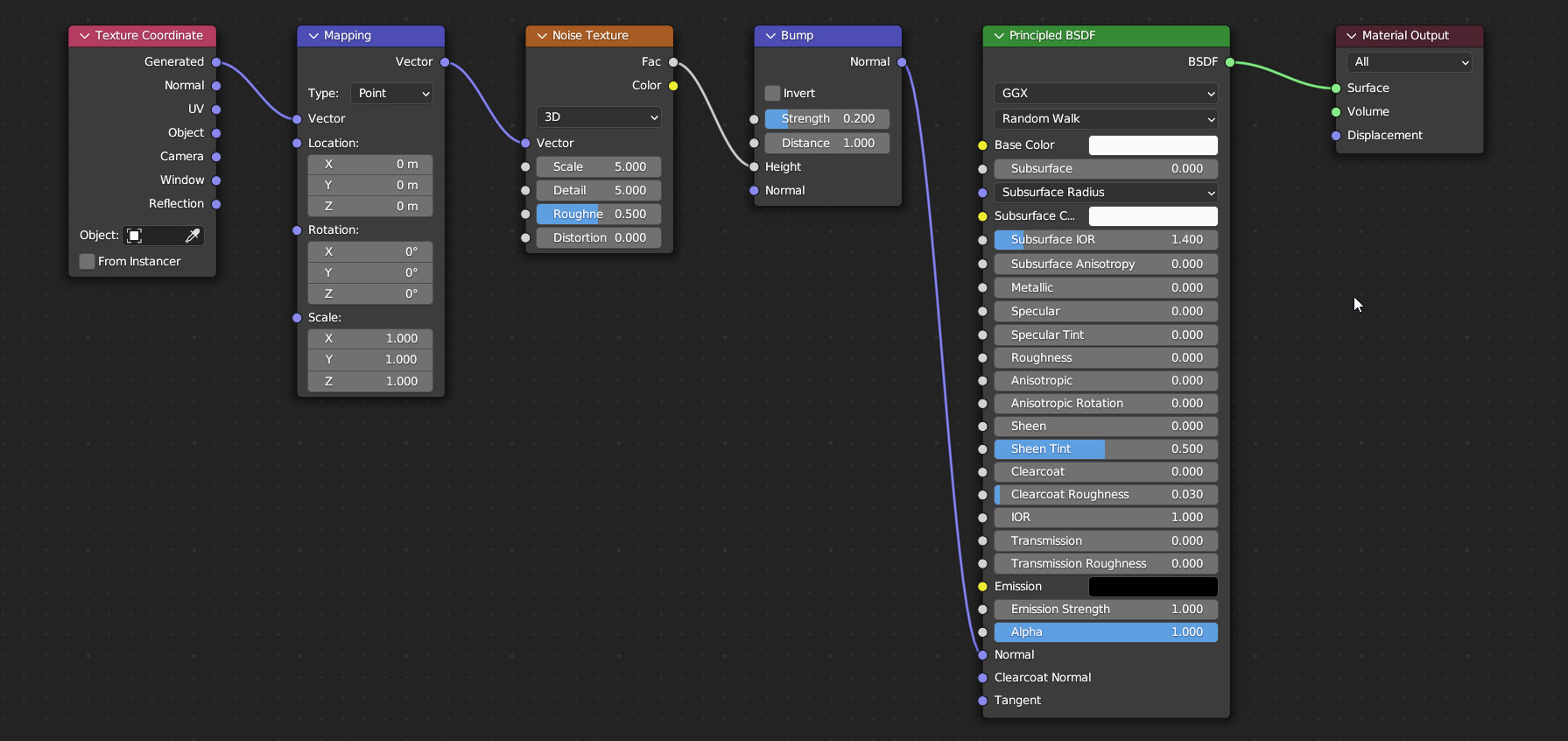
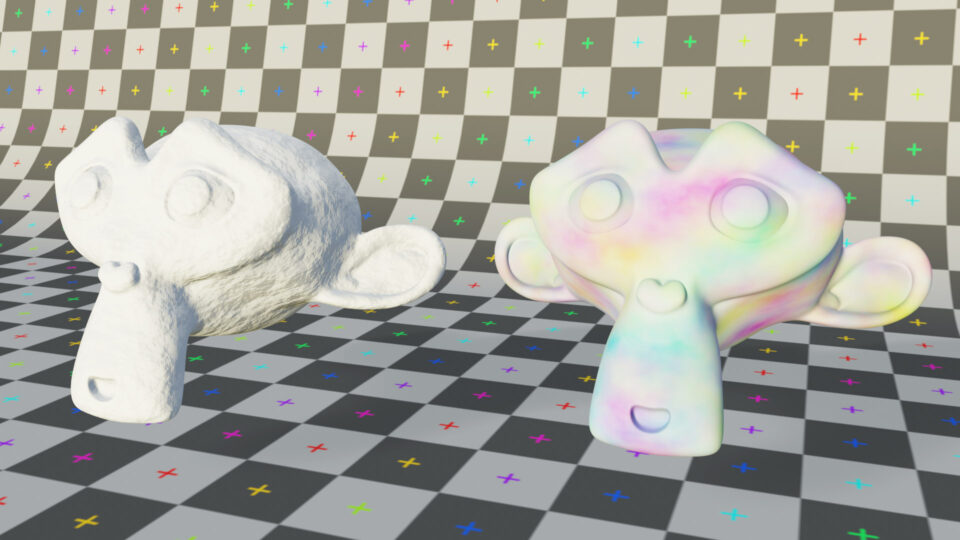
Noise is a texture that can be used to simulate random noise, more or less detailed, but also textures similar to clouds. The node has a Color output socket (yellow) and the usual Fac (gray). The bump node has three gray input sockets, of which the one that interests us is the Height parameter, in fact our intensity map (Noise texture) is connected precisely to the Height socket. The bump node has only the Normal output socket (purple – vector data) which in this case is connected to the homonymous socket in the Principled Shader. In the modeling section, we introduced the concept of normal, that is, the vectors perpendicular to each single face of the mesh; well, in this way the shading process varies the orientation of the normal along the surface in order to simulate the presence of reliefs (of any size) whose height is given by the height value indicated by our intensity map. The areas mapped with darker shades (if the Normal influence value is positive) correspond to indentations of the surface that will have maximum depth in correspondence with black (in the image below, the Suzanne mesh on the left). The bump node is therefore useful in creating small, but also significant reliefs, such as rough surfaces, floors, walls, etc. It is important to remember that in reality the geometry of the model remains absolutely smooth, which can be noticed by approaching the model from certain angles.
You can obviously experiment with other procedural textures and maybe combine them using MixRGB nodes (Color family) for color-type textures or the Math node (Converter family) for intensity maps.
The operation of the Mix RGB node is quite simple, we have two yellow sockets in input to which we can connect two textures (both procedural and bitmap images). Alternatively, we can also set a color in the respective rectangular areas.
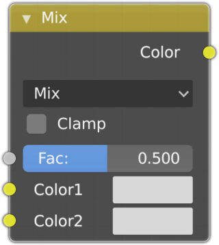
By clicking Mix, the Blend Type list appears, with the various blending methods that should be known to anyone who has used any photo retouching software. Mix performs a linear superposition: the value zero of fac will always prevail over the Color1 socket. You can also use any intensity map to vary the fac value:
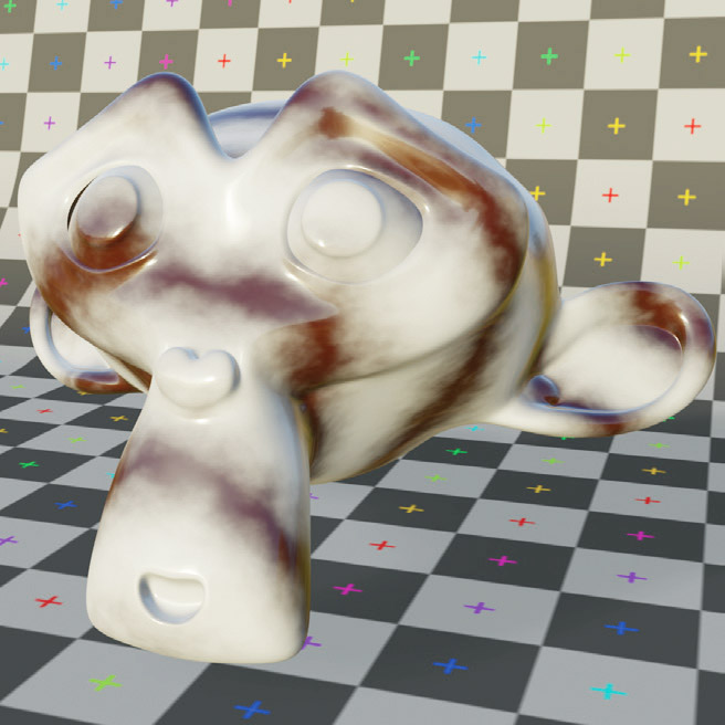
In the previous example, I connected the procedural Wave texture to the MixRGB node’s fac socket, so as to mix the white and brown colors according to the texture’s pattern. The result was then mapped to the Principled Shader’s Base Color socket. You can easily see that the possible combinations between textures and colors are practically infinite. In the image below on the page you can see how to combine two intensity maps through the Math node. The node is set to Add by default, so it proceeds to sum the values in the Value sockets. The Value output socket is connected to the MixRGB node’s Fac socket. So this time it will not be the only Wave texture used previously to regulate the mix of rgb colors, but the combination of it with the Musgrave intensity map.
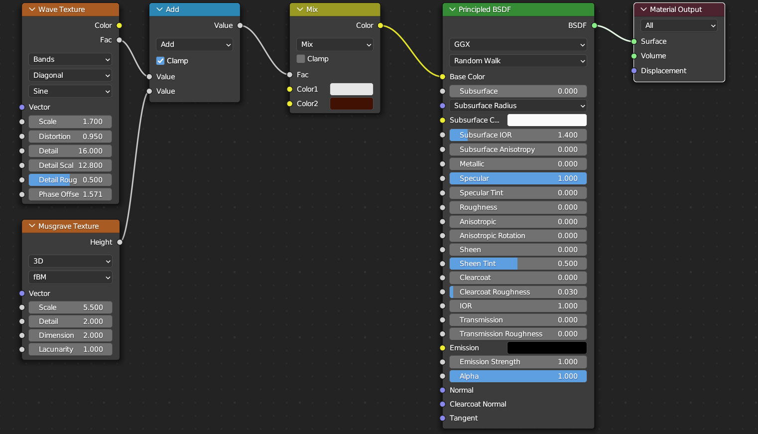
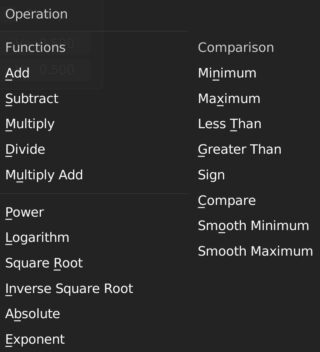
By summing two values that vary from 0 to 1, it is obviously possible to reach a maximum of two. Therefore, we can ‘normalize’ the operations performed by the map node so as never to leave the range 0-1, simply by activating the Clamp box. In addition to the sum, there are many other operations that the Math node can perform:
We will now move on to the extremely important use of Bitmap textures, which can be divided into two categories:
- Seamless images (tile, pattern, etc.), which will cover a large surface as desired when repeated.
- Images that require mapping to the model according to the rules of UV Mapping.
A seamless image is such that if applied repeatedly and alongside any surface, it will not show any signs of detachment or joint. When applying a seamless bitmap texture, we can use the Generated mapping coordinates, but we need to provide some more information to the software, for example indicating the projections to be used in the mapping process. In the following example and for all approximately cubic models (rich in edges) we will indicate Box in the third selector of the Image Texture node
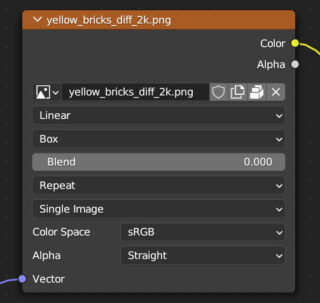
The default setting is Flat, which is great for all flat and open curved surfaces. Then there are the Tube projections (for closed, cylindrical-like curved surfaces) and Sphere (for models similar to spheres).
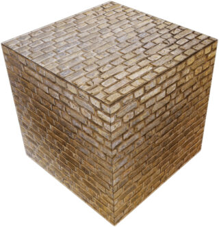
Let’s see the complete set of nodes used

We have a total of four Image Texture nodes for as many textures, of which the first (rgb) is connected to the base color, the second (black and white) to the specular socket, the third to the roughness socket (black and white), and finally the normal map. Let’s focus on the latter, which as you can see is connected to the Normal Map node. In the cube, in fact, there are grooves between the bricks that evee has shaded as if these were actually modeled. Many textures available online include so-called normal maps. There are also several software programs for generating textures and their normal maps, both commercial and open source.
Let’s see how a normal map is made:
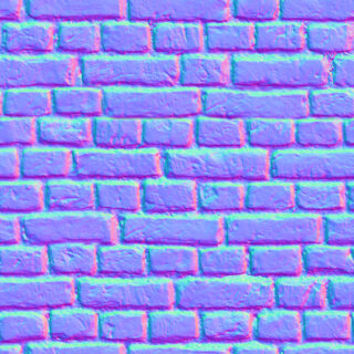
When we apply a normal map like this to the material, something very similar to what we saw earlier with the Bump node happens. The graphics engine will determine the shading of the surface as if its “points” (called Texels, or “pixels” in the Texturing process) had a normal different from the one perpendicular to the surface, thus realistically simulating the presence of small and medium reliefs. The normals useful for this purpose are derived from the RGB values of the pixels of the normal map and, being three-dimensional vectors, they require three components:
- The Red channel (0 – 255)
X component (-1.0 – 1.0) - The Green channel (0 – 255)
Y component (-1.0 – 1.0) - The Blue channel (0 – 255)
Z component (0.0 – 1.0)
Z therefore does not have negative values (i.e. normals facing inwards of the model), hence the reason why normal maps are mostly bluish bitmap images. In any case, such technical considerations are not of much concern to us and once you learn how to obtain the desired normal maps, or create them with special software (many of which are Free), their use as already seen will be very simple. When you download PBR textures, most of the time you will find compressed packages containing the following color (rgb) and black and white (b/w) images:
- diffuse map (rgb – base color)
- specular map (b/w -intensity map)
- roughness (b/w – intensity map)
- normal map (rgb)
- displacement (b/w – intensity map)
We will see displacement maps in action with Cycles because through them the engine will not only modify the shading, but it will also increase the polygonal detail of the surfaces. Intensity maps, being black and white images, do not require gamma correction, so in the Texture node it is necessary to set Non-Color in Color Space instead of the default sRGB profile (the same choice applies to normal maps although they are rgb images) ![]()
Next paragraph
Previous paragraph
Back to Index
Wishing you an enjoyable and productive study with Blender, I would like to remind you that you can support this project in two ways: by making a small donation through PayPal or by purchasing the professionally formatted and optimized for tablet viewing PDF version on Lulu.com