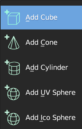
From the Add menu located in the header of the 3D view
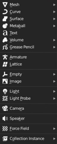
we can insert some basic shapes called primitives into the scene (both in object mode and within a model created in edit mode). Let’s start with the available mesh shapes:
- Plane
- Cube
- Circle
- UV Sphere
- Icosphere
- Cylinder
- Cone
- Torus
- Grid
- Monkey
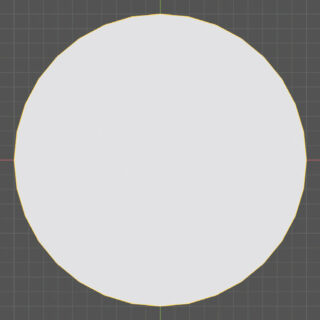
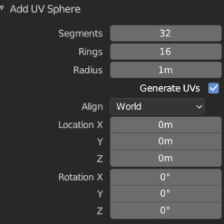
When adding the mesh shapes: Circle, UV Sphere, Cylinder, Cone, and Torus, a panel will appear to set the “definition” or detail of these objects. Performing any action other than modifying the parameters in this panel will make it disappear permanently. For the Circle primitive, we just need to decide the number of vertices, the radius, and whether to fill it using the options available in Fill Type or not (Nothing).
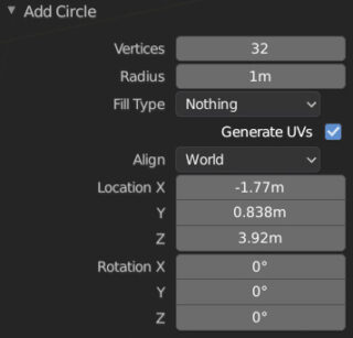
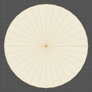
Filling is possible by choosing between Triangle Fan and creating as many triangles as there are vertices of the circle, or by treating the filled circle as an Ngon. In fact, more than a circle, we are talking about a regular polygon that is also useful in the case of needing pentagons, hexagons, etc. Finally, by setting Align>View (option available for all primitives), the circle will automatically orient itself to the perspective of the 3D View.
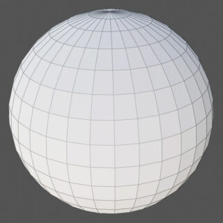
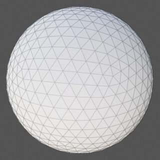
For the UV Sphere primitive, it is also necessary to set a resolution by setting the number of vertical segments with the Segments value and the number of horizontal segments with Rings (typically, Segments is twice as many as Rings). Icosphere is an approximately spherical polyhedron with triangular faces, whose resolution is controlled by the single Subdivision parameter.
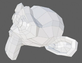
Cylinder, Cone, and Torus have settings that are completely analogous to those just described. A mention should be made of the Monkey primitive, called Suzanne, which is the mascot of Blender: a model that is neither complex nor simple, and which is often useful for testing various types of modeling techniques or the rendering of materials through test rendering; an object that is nothing if not essential in the learning phase of the software and which will therefore often appear in these pages.
Objects inserted into the scene in this way are placed so that their center coincides with the position of the 3D Cursor. For the Cube, Cone, Cylinder, UV, and Ico Sphere mesh types, it is possible to use the Add tool located at the bottom of the toolbar.

Activating it will cause a white circular grid to appear in the 3D View that will move on either the plane defined by the global xy axes (z=0) or on the surfaces of any other meshes already present in our scene.
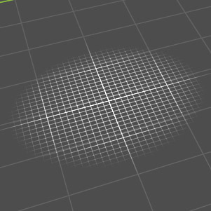
Overall, the operation is quite intuitive and it is easier to understand by testing it in the field rather than explaining it in words. Using the left mouse button will define the base (you can use the Alt and Caps Lock keys to center and proportion the base), after which the height will be defined.
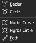
We now arrive at the rich family of curves and surfaces. Unlike meshes, which are fundamentally defined by their vertices, curves and surfaces are geometric entities described by mathematical functions. This topic will certainly be familiar to anyone who works with vector graphics, in which case it will just be a matter of getting used to the implementation of these tools in Blender by including the third dimension in your experience; without forgetting that Blender allows the import of the Scalable Vector Graphics (SVG) format. The mathematical nature of these objects makes the software technology necessary to integrate them into 3D graphics applications rather complex; it is enough to consider that NURBS curves (generalizations of Bézier and B-Splines) have a technical reference volume of 645 pages. Fortunately, Blender allows us to use them profitably after just a few hours of experimentation. Curves are divided into Bézier and NURBS, the difference being that the first are modeled through interpolation and the second through attraction. In Blender, Bézier curves are also used to define the interpolation between two keyframes in the animation process of any element of the 3D scene.
The complete list of available curves can be found in the Add menu>Curves (3D View header).
Let’s immediately analyze a Bézier curve in a 2D context by positioning ourselves in the Top Ortho view. In edit mode, the curve appears divided into some main points (or control points) through which the curve itself passes.
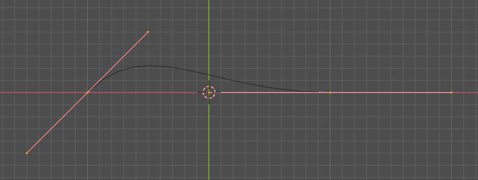
These points are sensitive to the same transformations seen for the vertices of meshes (translation, duplication, extrusion). In addition to this, we find two other points at the ends of the segment tangent to the curve at each of its control points (segments that can be translated, scaled, and rotated); these are the “handles” useful for modifying the shape of the curve. To extend the curve, simply extrude (E key) one of the two control points at the ends.
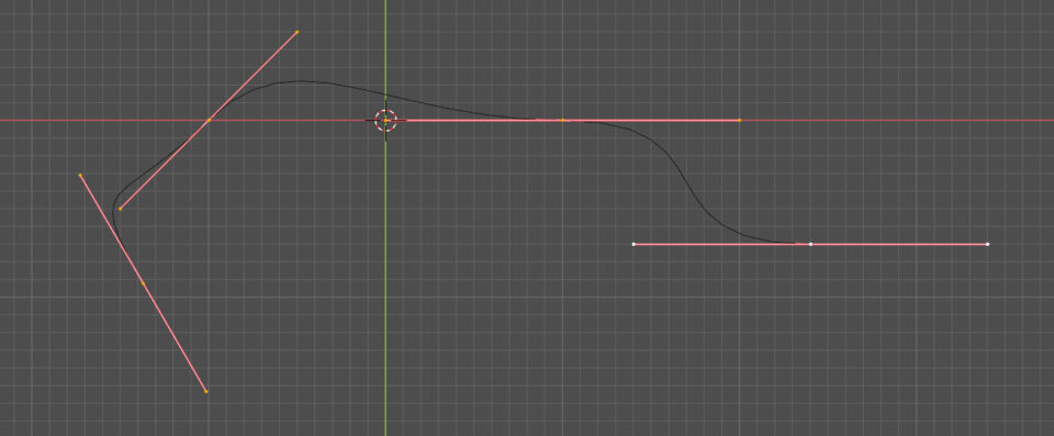
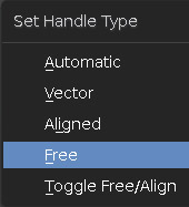
By moving one of the two handles, you will notice that the other will position itself so that both remain aligned along the segment that connects them (this is the default Align mode); we can move these points individually to create cusps, in this case just select the handles and press the V key to bring up the Set Handle Type window where you can choose Free, then Aligned to return to the previous state.
The Automatic mode allows you to more easily draw smoothly rounded and polished curves, while Vector is useful for drawing broken lines. The density of the main points may not be uniform along the curve and may vary depending on the shape you want to achieve. After selecting two contiguous control points, you will get N additional intermediate points by using Subdivide.
The operation of Nurbs (Non Uniform Rational Basis-Splines) curves is more intuitive, as their control points define a broken line that attracts the various arcs of the curve towards itself. By extruding one of the two outer points, we increase the complexity and length of the curve
In the examples shown above, we kept the curves flat by modifying the position of their control points from the top view, but it is possible to translate the various points in the third dimension (z) as well, creating curves that wind freely in space. In fact, going to the Object data properties menu, in this case marked by the icon ![]() , in the Shape panel we immediately see that by default the curve is of type 3D.
, in the Shape panel we immediately see that by default the curve is of type 3D.
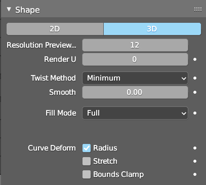
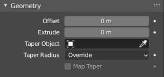
By clicking 2D, the points of the curve will instead be translated so that they all belong to the same plane. By using curves, it is possible to obtain various types of surfaces using extrusion. In the Geometry panel, the Extrude parameter adjusts the extrusion from 0 to any value. Extruding will result in a surface whose edge is the starting curve.
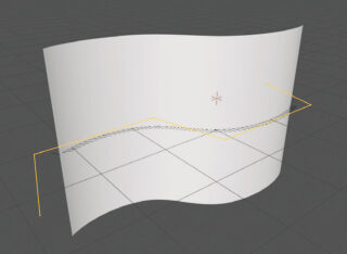
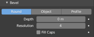
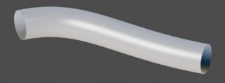
Subsequently, we can round the edges of the extruded curve by varying Depth in the Bevel panel and round them more by increasing the Resolution value. The behavior of Bevel depends on the choice made in Fill (filling) located in the Shape panel (we are talking about 3D curves): Half (half filling) makes the curve (or the edge of an extruded curve) closed halfway with a circular profile defined in Resolution.
Full returns a cylindrical surface around the shape of the curve defined in edit mode: this is a possible way to easily create models of pipes or electronic cables.
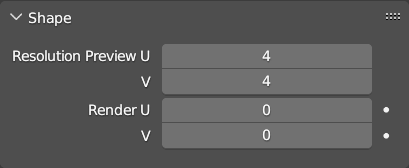
In the Shape panel we find the Resolution Preview U option related to the degree of approximation of the real-time graphic representation of the curve which is set to 12 by default. In Render U the default value is Zero, which maintains the precision set in the viewport also during the final rendering, but it is possible to increase this value to obtain almost perfect curves (at the cost of longer processing times). The resolution set for the preview is also important for another reason: by transforming the curve into a mesh (from the Object Context menu -> Convert to of the 3D View in object mode) the degree of accuracy of the final mesh will be exactly that obtained with the resolution value chosen in Preview.
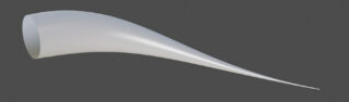
A powerful modeling method is to obtain surfaces by extruding a curve through the profile of another curve, using the Taper Object (Geometry panel) and Object (Bevel panel) fields. The following image shows a Bézier curve with a simple Circle-Bézier as its bevel object.
Therefore, the surface can be tapered using a second Bézier curve in Taper Object:
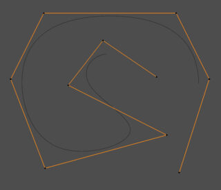
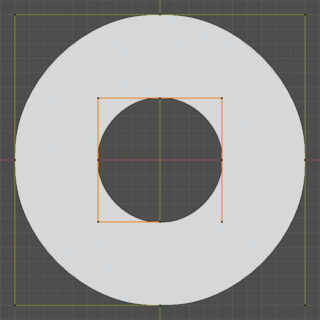
In edit mode, you can test the following interesting property of closed and filled 2D curves (to make any closed flat curve filled, simply set Both in the Fill Mode field in the Shape panel). By inserting one curve inside another, a “holed” topology is created. For example, starting from a closed nurbs circle (closed), we just have to insert (as already mentioned in edit mode) another circle and scale it to your liking with the S key, having first selected its control points. The same goes for Bézier curves.
In edit mode, the toolbar displays tools for modifying our curve such as the extrude we have already discussed. Let’s now focus on the excellent Draw tool (the first at the top) that allows us to draw our Bézier curves directly in the 3D view.

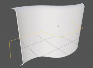
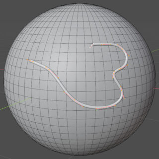
The curve can be drawn with a single, prolonged left click of the mouse, or more conveniently using a graphics tablet. The sections of the curve thus created will belong by default to the plane orthogonal to the point of view and passing through the 3D Cursor; but there is a different option that allows us to model the curve on any mesh. Let’s see a practical example by inserting a Bézier curve and a sufficiently detailed UV Sphere (64 Segments for 32 Rings) into our scene. In edit mode, we select and delete all the control points of the Bézier curve (X>Delete Vertices) so we are left with an empty curve; always in edit mode, we start the Draw tool and in the Tool tab of the sidebar menu (N key) we select Surface in the Depth field.
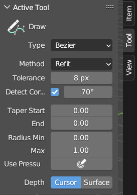
In the Object Data properties context, we set the Resolution Preview U to 24 and then select Full in Fill Mode (default setting). Finally, in the Geometry panel, we give a Bevel>Depth of 0.015 m with 5 resolution (so we can see the 3D shape of our curve). At this point, all we have to do is draw directly in the 3D View on top of the sphere and see the curve adapt to the shape of the mesh. In the image on the bottom right, the result of a curve drawn on the surface using the pressure levels of a graphics tablet is visible. We can also taper the ends of the sections of the curve by inserting different values from zero in Tapers Start/End.
In the Show Overlay menu, icon ![]() you will find at the bottom the box for the Normals option.
you will find at the bottom the box for the Normals option.
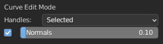
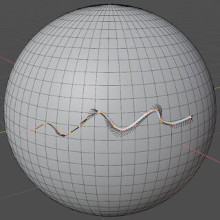
By activating it, you will notice that in edit mode the curve has an orientation defined by arrows, which will be useful when we talk about animation.
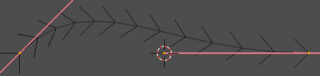
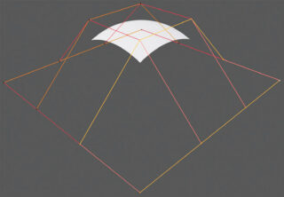
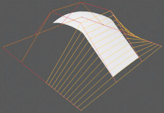
In a completely analogous way to Nurbs curves, we can begin to experiment with Nurbs surfaces, for which the control points will be the vertices of a three-dimensional matrix rather than belonging to a broken line.
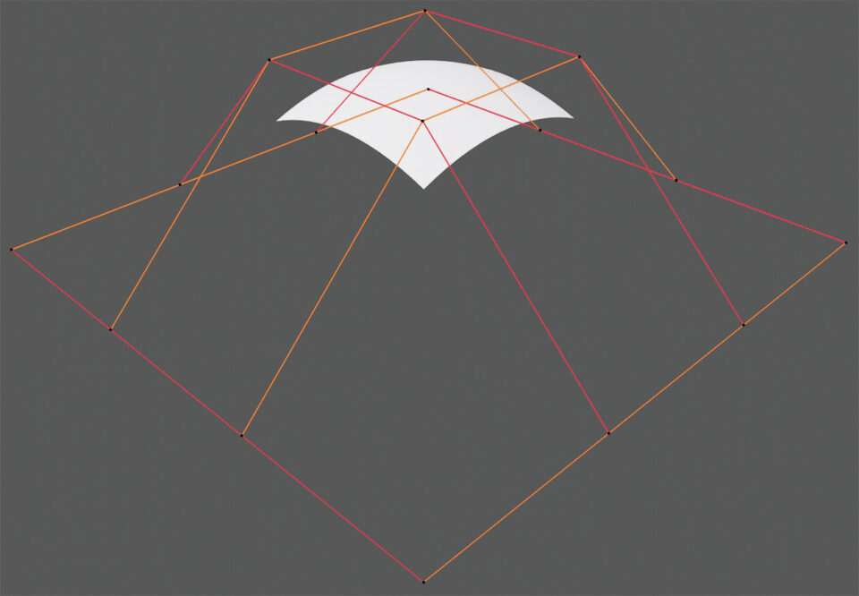
To extend the Nurbs surface, increasing its detail, just select the vertices of one of the outer edges of the control matrix and extrude them with the E key.
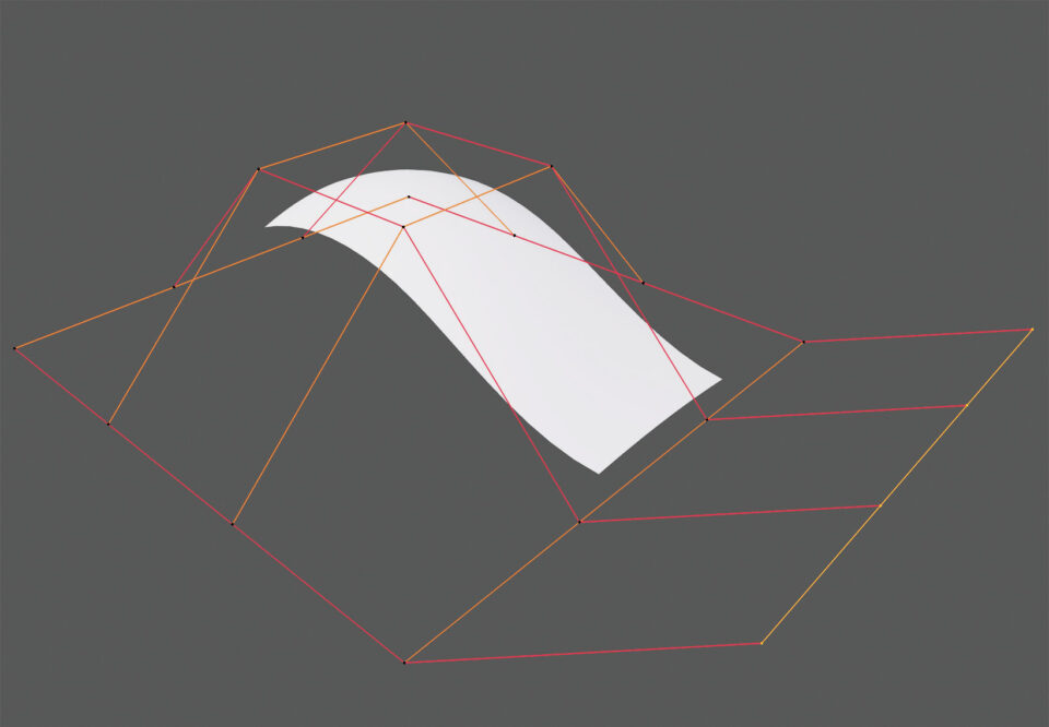
Subdivision is possible by selecting all the vertices of the matrix that make up a complete “strip”, from one edge of the matrix to the other, as shown in the images below, or by selecting all the vertices with the A key.
For NURBS surfaces, the parameters of the Shape panel are double the number seen for curves, we will in fact have one for the U division and another called V (also known as UV mapping coordinates). Try to imagine these surfaces as a fabric that you can always “stretch” into a flat shape, in this case with the U and V parameters we will decide the quality of the resolution in its two dimensions. In the same exact way as previously seen we can transform the surface into a mesh, with the degree of approximation set in resolution.
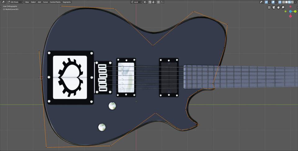
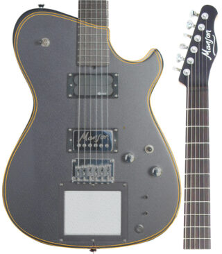
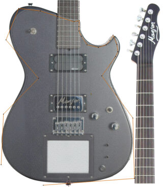
Now let’s see the example of the body of an electric guitar that shows how curves can be a powerful modeling tool, perhaps along with the technique mentioned at the end of the previous paragraph, that is, using a background image in the orthogonal views (some renders of this model are visible in paragraph 4.1).
In the Add>Surface menu, in the header of the 3D View, we also find Bézier and Nurbs surfaces in the form of circles, spheres, cylinders, and toroids, for which the same rules apply as previously explained.
Next paragraph
Previous paragraph
Back to Index
Wishing you an enjoyable and productive study with Blender, I would like to remind you that you can support this project in two ways: by making a small donation through PayPal or by purchasing the professionally formatted and optimized for tablet viewing PDF version on Lulu.com